Creating a Custom Profiling Target for Scanners and Cameras

2010-12-19

---

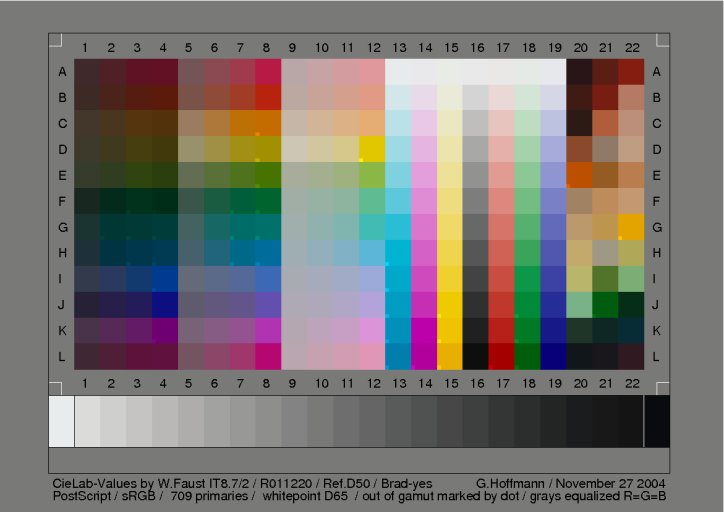
When generating a colour profile for a scanner or camera there are several standard targets that are traditionally used. The most widely-recognised of these is probably the IT8.7/2 chart, with its spread of greys, synthetic colours and real-world shades. There are other options too, such as the ColorChecker DC or SG charts, but what if you want to create your own chart?

---

It’s perfectly possible to do this, and there are several reasons why you might want to. You might, for instance, be unable to eliminate reflections at a particular position so want to use a matte rather than gloss target. Or perhaps you want to use a target with a brighter white than the off-the-shelf targets offer in order to avoid clipping of paper texture when scanning in a piece of artwork (see also Argyll's -u and -U switches for colprof if this is an issue for you) – or maybe you want to create a profile that uses a custom illuminant, or perhaps you want to eliminate inter-instrument disagreement as a source of inaccuracy when printing scanned images.

While there are good reasons why you might want to use a custom target there are also good reasons not to - namely that the target's gamut is of course limited by that of your printer (and likely to be somewhat smaller than professionally-produced targets), and also a home-produced target is likely to exhibit more problems with metamerism (where colours that match under one set of viewing conditions fail to do so under another).  If you want to try creating a custom profile despite these potential issues, read on!

To generate an ICC profile for a camera or scanner using ArgyllCMS you need:

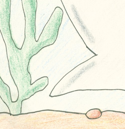
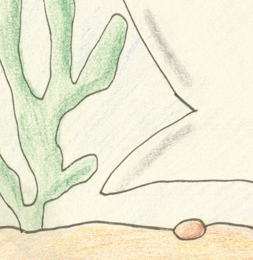
• A profiling target

• A .cht file describing the patch layout

• A reference file, describing the physical colour of each patch on the calibration chart.

Argyll comes with .cht files for the common targets, and the targets themselves are supplied with suitable reference files – but obtaining these files for a custom target is a little bit trickier.

To follow this guide you will need the following:

• A scanner or camera to profile

• A printer with good repeatability and good colour consistency across the page. Pretty much any recent inkjet printer in high-quality mode will do, but laser printers are less suitable since they generally have significantly worse repeatability.

• A spectrophotometer supported by ArgyllCMS, such as a DTP41, an Eye-one Pro or a ColorMunki.

• ArgyllCMS 1.3.0 or newer.  (Older versions may work, or may fail to read the reference file we create later on - I haven't tested.)

The first step is to generate the patches themselves. We use targen in RGB print mode, like so:

> targen -d2 -g30 -f376 Tutorial

Here we’re asking for Print RGB, 30 grey patches, 376 patches in total.  You can, of course, use any patch specification you like - this is just an example.

As mentioned previously, to use a custom target for profiling a scanner or camera we need both a .cht file and a reference file.  Obtaining the .cht is easy, because Argyll will generate one if we ask it to render the target in a form suitable for reading with a scanner:

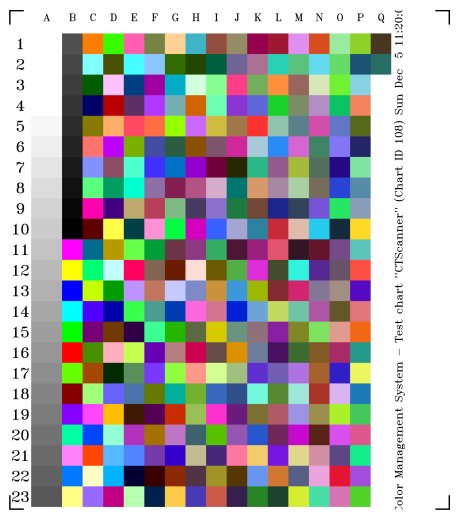
> printtarg -t300 -p150x185 -r -s -iss Tutorial

We’re asking for 8-bit TIFF rendered at 300dpi, to fit a page 150x185mm. (The actual size doesn’t matter, I just used these dimensions to get the shape I wanted.) The -s parameter tells printtarg to generate a .cht file, and -iss indicates that the patch layout should be suitable for a scanner (Reading via a scanner uses the same layout as a SpectroScan, which is what the "ss" stands for.)  The -r parameter tells printtarg not to randomise the patch locations - this is important for a reason that will become clear later on.

We now have a TIFF file, Tutorial.tif, that we can print out to serve as our target, but unfortunately this printed target isn’t suitable for reading by a DTP41, Eye-One or ColorMunki. To get around this problem we need to print the exact same set of patches a second time, this time in a layout the spectro can handle. This is why you need a printer with good repeatability.

Copy the Tutorial.ti1 file to a new file, TutorialRef.ti1, then do this:

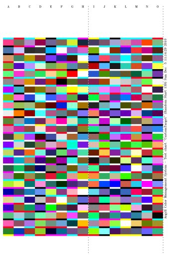
> printtarg -i41 (or -ii1 or -iCM depending on your instrument)
       -pA4 (or Letter, or whatever) -t300 TutorialRef

Again, we have a 300dpi TIFF suitable for printing. This file must be printed on exactly the same type of paper using exactly the same print settings as the scanner target.

Give the printed page time to stabilze – ideally at least overnight – then read it in using chartread.

We now have TutorialRef.ti3 containing the information we need for our reference file.

Firstly we’ll get rid of the spectral measurements, using spec2cie

> spec2cie -n TutorialRef.ti3 TutorialRefCIE.csv

(You can also specify FWA correction options and custom illuminants if you so wish.)

All that remains is to massage the newly-created file so that scanin can use it.  What we need to do is to replace the patch names in our new TutorialRefCIE file with the patch names from the scanner target.  Because we used the -r paramter when generating the scanner target, the patches in the Tutorial.ti2 file are in the same order as in the TutorialRefCIE.csv file, even though the patch names are in random order in the latter file.

The easiest way to transplant these values is to open both the Tutorial.ti2 and TutorialRefCIE.csv files in OpenOffice Calc.  This is much easier if the filenames end in .csv, so copy the .ti2 file and change the copy's file extentsion to .csv.

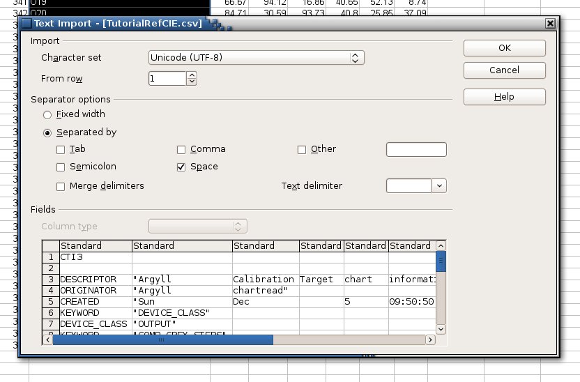
When importing the files, you'll be asked for CSV import options - it's important that you uncheck "comma", check "space", and remove the quote mark from "Text Delimiter".  Once both files are open, find the list of patch names from Tutorial.csv, starting at A1 and continuing until the end of the file, highlight just that column of patch names and copy it to the clipboard.

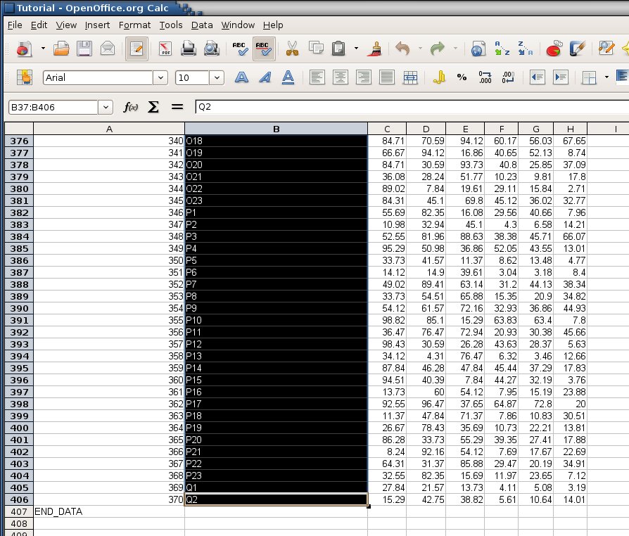
Now, in TutorialRefCIE.csv, find the first patch name (which, because this file used random layout, could be anything), place the cursor on that cell, and paste the clipboard.  You should have now replaced the patch list with a neat alphabetically-sorted one which will match up with the scanner target.

There's one last thing to do - at the head of the file find and delete the line which reads

SPECTRAL_BANDS "31"

(The actual number depends on which instrument you used.)  The presence of this line causes problems with scanin, so we just delete it.  It's no longer relevant anyway, since we stripped the spectral data earlier using spec2cie.

Click save, and reassure OpenOffice that you do want to save in the original CSV format.

 

To use the newly-created target to profile a scanner, scan in the printout of Tutorial.tif, and save the scan as, for example, Scanner.tif - then do this:

> scanin Scanner.tif Tutorial.cht TutorialRefCIE.csv

You should now have a .ti3 file called Scanner.ti3, and you can generate your profile, as usual, with:

> colprof -D”Profile Descriptive Name” Scanner

You should now have a profile called Scanner.icc (or .icm if you're on Windows), generated using your custom target.